For the thoughts of mortals are timorous, and our devices are prone to fail.
The Wisdom of Solomon ch. IX, The Apocrypha.
The cost model in chapter 5 requires a knowledge of scan time for range queries. This chapter investigates the relationship between query size and number of partitions accessed (and hence scan time) in a single dimension.
A new formula describing the number of partitions accessed by large range queries in files which do not have a large number of range partitions is developed. Comparisons are made between this and a related formula defining the number of pages accessed by range queries. A rather interesting new observation is that for the case of a file with a very small number of partitions, the query size, in addition to the number of partitions, affects the scan time reduction that can be obtained by further partitioning.
The number of partitions accessed by queries must be known (in order to determine scan time [footnote 5]). In the case of single data valued (sdv) partitions the analysis is simple.
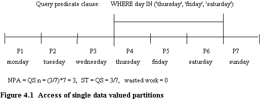
Consider a file range partitioned on a low cardinality attribute, such as "day_of_week", so that records with a given attribute value are stored in different partitions. For convenience, assume there is an even data distribution. Since query predicate values must coincide with partition boundary values, the number of partitions accessed (NPA) by a single range query, NPAsdv, is given by
NPAsdv = QS.n (4.1)
Where QS refers to the query size (or query selectivity) expressed as a fraction of file size, and n is the number of partitions. This is exemplified in figure 4.1
The scan time is simply
STsdv = QS (4.2)
In practice scan time will depend upon the amount of data within the accessed partitions. Assuming the data distribution is known, the proportional scan time can be determined.
The wasted work done in resolving MIS range queries is zero in all cases.
In the case of partitions that can hold many possible data values analysis is more complex, because query predicate values are not guaranteed to coincide with partition boundary values. Thus in the first case, in order to determine an appropriate number of partitions for a column we are led to analysing how the average scan time of a set of range queries of a given size varies with number of partitions.
As a starting point, Eastman's formula [EAST87] for the number of pages accessed by range queries was applied to the calculation of number of partitions accessed. It is simple to show that when the number of partitions, n, is small, the formula gives incorrect results, although it holds when n is large. It also implies that scan time reductions due to further partitioning are independent of query size. First Eastman's formula, which is called the approximate formula, is reviewed and then a more accurate model is derived. These are discussed in the light of scan time reductions between n and 2n partitions.
For the purposes of derivation of the formulae, a single partitioning column (dimension) only is considered, and it is assumed that the domain of this is large. Further assumptions are that partitions of a given dimension contain approximately the same number of records and that there is an even data distribution on the partitioning column. In practice an even data distribution is unlikely. However, if the data distribution is known for the partitioning column, then a mapping between the observed query predicate, and the actual query size (i.e. the proportion of records referenced by a query, also known as selectivity) can be made. Conversely, using the cumulative data distribution, partition boundaries can, in most cases, be derived which ensure partitions contain approximately equal numbers of records (thus for practical purposes data distributions of the partitioning columns must be relatively stable).
Eastman [EAST87] states that on a single partitioning dimension of a range partitioned file where the data buckets (pages) are of equal size and where all the queries are of the same size, the average number of pages accessed by a set of range queries is
average number of pages accessed per query = 1+s/d (4.3)
where s is the size of the queries, and d is the size of the unit of access (i.e. data page), both expressed as a fraction of the domain size. For example, assuming that each query references 0.145% of the records in a range partitioned file, and assuming that there are 10,000 data pages, then the size of the queries is 0.00145 (i.e. 0.145/100), and the size of each data page is 0.0001 (i.e. 1/10,000). The number of pages accessed on average by a set of these queries will be 15.5 (i.e. 1+0.00145/0.0001). Of course, each individual query will access a whole number of data pages. Note that the actual range query predicate values are not needed - what is important is the magnitude of the queries. In section 4.3 a derivation of equation (4.3) is presented.
Because of the granularity of the IDIOMS MIS partitioning strategy, some of the explicit and implicit assumptions underlying the derivation of equation (4.3) no longer hold, and it ceases to provide an accurate description if it is used for the number of partitions accessed. This is shown by the following example.
Let the number of partitions, n, = 4, and let s = 0.8
hence d = 0.25, since 1/number of partitions = partition size
average number of partitions accessed = 1 + 0.8/0.25 = 4.2
But there are only four partitions. Accordingly, a more accurate model for the number of partitions accessed is derived in section 4 of this chapter.
One implicit assumption underlying equation (4.3) is that the number of buckets (i.e. units of access) in a given dimension is large, and this leads to errors when equation (4.3) is used to estimate the number of partitions accessed. For MIS purposes 20 partitions in a given dimension is probably sufficient (see chapter 5 - cost model, and chapter 6 - example). Since there are no indices for MIS queries, a data partition is the unit of access for these queries (OLTP queries access data at the page level). Where n is very small, large MIS queries can result in access to all partitions, whatever the query predicates associated with a query of given size. This is exemplified in figure 4.2, where each horizontal line represents a query of selectivity 0.8. For a query to have a selectivity of 0.8, the lower bound of the query predicate must range between 0 and 0.2 (for convenience a numerical domain is assumed, which ranges between 0.0 and 1.0). In cases such as this, the minimum, maximum, and average number of partitions accessed are all equal to the total number of partitions on that column.
However, this is not the only source of error. Recall we are dealing with the average number of partitions accessed by a set of queries of identical size. On an individual basis, some queries will access a minimum number of partitions and others will access a maximum number of partitions, dependent upon the query predicates and the partition boundaries. The proportion of records accessing the minimum and maximum number of partitions varies with the size of queries and the number of partitions, and this needs to be accounted for. As a convenient term to express this the label "end effect" is used (see section 4.4).
The derivation of the average number of partitions accessed, avgNPAexact, is shown in two stages, the first, avgNPAapprox, corresponding to the approximate formula presented in Eastman [EAST87]. Then in section 4.4 this approximate formula is used to derive an exact formula to deal with the problem of "end effect" and large queries. In order to make a distinction between Eastman's number of pages formula, and the formulae derived in this thesis different terminology is used.QS refers to query predicate size (or query selectivity, due to the mapping between observed query predicate values and true selectivity), and PS refers to partition size (QS and PS are equivalent to s and d respectively in Eastman's terminology).
Consider a set of range queries, all of identical size, QS, with the range boundaries evenly distributed throughout the domain range. The diagonal lines of figure 4.3 represent the lower and upper range predicate values of a large set of range queries of (a given) identical selectivity.
The minimum number of partitions accessed, minNPA, by a single query is éQS.nù because a partition is either accessed or it is not, hence we always round up, indicated by the symbol é ù. All queries with a predicate lower boundary value greater than or equal to point a and less than point b in figure 4.3 will thus require access to the minimum number of partitions (two in the example, shown shaded light). All queries with a lower boundary value greater than or equal to point b, and less than point c will access the maximum number of partitions (shown shaded dark) that a query of that size is able to access (i.e. minNPA + 1). In other words, the distance a to b represents the proportion of queries which result in access to the minimum number of partitions, and the distance b to c represents the proportion of queries which result in access to the maximum number of partitions.
If the lower bound of a range query predicate is greater than or equal to c, similar considerations apply as in the cases above, though on a different set of partitions.
notes on figure 4.3
The approximate average number of partitions accessed, avgNPAapprox, ignoring "end effect" and the problem of large queries, is given by
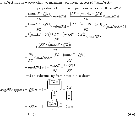
This is equivalent to 1+s/d, where s is the size of a query, and d is the size of a partition (recall d = 1/n).
Equation (4.4) is derived under the implicit assumption that there will always be a constant proportion of minimum and maximum partition accesses. This is not true, except in the case that the query size is some multiple of the partition size. The "end effect" described in section 4.2 becomes prominent when n is small and QS is large. This is shown in figure 4.4, which has 6 partitions, and a set of queries of size QS = 0.36.
Note: the meanings of abbreviations can be found under figure 4.3.
Figure 4.4 is based on figure 4.3, but it deals with the cases where
a) query size is not a multiple of partition size and
b) minNPA = maxNPA.
The subset of queries with a predicate lower boundary value greater than or equal to point a and less than point b will access on average avgNPAapprox partitions, as defined by equation (4.4). Note that point b will always fall on the lower boundary value of some partition.
Those queries with a predicate lower boundary value greater than or equal to b and less than or equal to c must always all access the minimum number of partitions, minNPA.
The distance a to c (i.e. 1-QS) represents the range within which a query predicate lower boundary can be found. Thus the exact value of the average number of partitions accessed is defined:
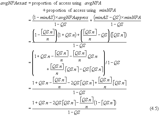
When QS=1, we know that all the partitions are accessed (i.e. éQS.nù = n). However, due to the denominator (1-QS), division by zero occurs. Thus strictly, the correct formula is given by
![]()
When the assumption underlying the derivation of equation (4.4) holds (i.e. QS is a multiple of PS; éQS.nù = QS.n) equation (4.5) reduces to equation (4.4), as shown below.
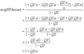
The formulae above refer to partitions accessed, but in order to make comparisons between levels of partitioning, it is convenient to use (proportional) scan time. Average scan time is simply the average number of partitions accessed, expressed as a fraction of the total number of partitions. For convenience, equation (4.5) is used in the following discussion with the understanding that if QS = 1, we know that avgNPAexact = n, and average scan time = 1.
![]()
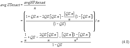
Intuitively we might expect QS as well as n to affect scan time differences, ΔST>n,m, between two levels of partitioning, which is defined simply as
ΔST>n,m = STn - STm (4.9)
Here consider scan time differences between n and 2n.
Using equation (4.7) to define scan time differences, we find that query size plays no part.

This does not model correctly the situation when n is small, as shown in table 4.1, which shows scan time differences between 3 and 6 partitions (ΔST3,6) for some arbitrary values of QS. Percentage differences between ΔST3,6 and the value of 1/2n (0.167) are also shown, labelled as %difference. Scan time was determined using equation (4.8).
| QS | 0.05 | 0.15 | 0.30 | 0.50 | 0.80 | 0.90 |
|---|---|---|---|---|---|---|
| scan time, n=3 | 0.368 | 0.451 | 0.619 | 0.778 | 1.000 | 1.000 |
| scan time, n=6 | 0.211 | 0.314 | 0.460 | 0.667 | 0.944 | 1.000 |
| Δ ST3,6 | 0.158 | 0.137 | 0.159 | 0.111 | 0.056 | 0.000 |
| %difference | 5.8 | 21.7 | 5.2 | 50.3 | 200.6 | undefined |
| %difference refers to the difference between Δ ST3,6 and Δ STapprox3,6 | ||||||
Now ΔST3,6 as defined by equation (4.10) equals 0.167 (i.e. 1/(2×3)), which does not show the variation in ΔST3,6 with differing QS. However, using the improved formula describing average scan time, equation (4.8), we see that QS does indeed make an appearance.
There are two formulae describing ΔSTexactn,2n depending on the relationship between QS and n. This is because
case A: when QS \ PS ≤ PS/2 and QS \ PS > 0, then éQS.2nù = 2 éQS.nù - 1
case B: when QS \ PS > PS/2 or QS \ PS = 0, then éQS.2nù = 2 éQS.nù
(The operator \ symbolises modulo reduction; a \ b is the remainder when a is divided by b).
We cannot take an average of these because of the inherent "end effects" - at least as far as large QS and/or small n is concerned.
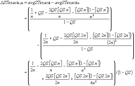
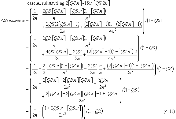
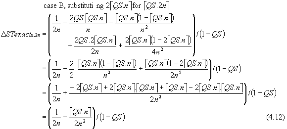
When QS is a multiple of PS (i.e. QS \ PS = 0; éQS.nù = QS.n), equation (4.12) reduces to equation (4.10) because the assumptions underlying the derivation of equation (4.4), from which (4.7) and (4.10) are derived, hold by definition.

In the final section of the chapter comparisons are made between results obtained from the new formulae, and those from the approximate formulae.
Figures 4.5 and 4.6 show values obtained using the approximate and exact formulae (indicated as approx and exact on the figure legends) for average number of partitions accessed and average scan time respectively, for three arbitrary query sizes. Although the curves are seen to converge for all query sizes, where the number of partitions is small and QS is large some serious differences appear. This is seen clearly in figure 4.7, which shows percentage differences between results obtained using the exact and approximate scan time formulae, equations (4.8) and (4.7) respectively. For some values of n the two formulae give identical results (e.g. QS = 0.9, n = 10), and as discussed previously, this occurs when QS \ PS = 0. (It is perhaps unfair to criticise the approximate formula for the errors in the case where n = 1, since we know that the number of partitions accessed must by definition equal 1, and the scan time must equal a full file scan).
In some ways the findings are negative; by making a simple (and common sense) modification to the approximate formulae for number of partitions accessed and for scan time, equations (4.4) and (4.7), we are able to overcome the gross errors (i.e. partitions accessed > total number of partitions, n; scan time >1) which occur. The modification is to limit the calculated value of partitions accessed to n (and similarly for scan time, limit the result to 1). Thus
avgNPAmodified = min(n, (1 + QS.n)) (4.13)
avgSTmodified = min(1, (1/n + QS)) (4.14)
As an example, percentage differences between results obtained from the exact formula, equation (4.8), and equation (4.14) are shown in figure 4.8, which is on the same scale as figure 4.7 for ease of comparison. It is interesting to note how for large queries, the errors all but disappear. For scan time estimation purposes the errors that remain for small queries are probably acceptable even for small n.
Figure 4.9 shows the scan time differences between n and 2n. There is a curve showing the approximate value of ΔSTn,2n, as defined by equation (4.10), and hence it is labelled 1/2n on the legend. The three curves for the representative values of QS are seen to converge towards 1/2n. The values were obtained by using equation (4.8) (i.e. avgSTexactn - avgSTexact2n), rather than actually using equations (4.11) and (4.12) to calculate ΔSTn,2n. Percentage differences between the exact and approximate values of ΔSTn,2n for the three representative values of QS are shown in figure 4.10. The values of QS were not chosen to produce the most dramatic results. For example, a QS of 0.87 when n = 4 results in an difference of 1200% (!) between the exact and approximate result. The use of ΔSTn,n+1 as metric for partitioning is considered in chapter 5, and it is interesting to note that in general the errors in this case are far greater than those for ΔSTn,2n.
One assumption that is made both in this work and by Eastman is that the range queries (of any given size) are evenly distributed. This is not guaranteed, and it is possible that some regions of the domain are referenced more frequently than others. Furthermore, partition boundaries may be overlapped in a non-uniform manner. For practical purposes, this is of no concern to partitioning decisions for scan time reduction (although of course, there are issues of load balancing to be considered) since the absolute magnitude of scan time reduction is of interest (see chapter 5). Recall that the minimum number of partitions accessed by a single query is given by éQS.nù, and the maximum number of partitions is éQS.nù +1 (or n, when éQS.nù = n). Thus for any set of queries of a given size, whether they all access the maximum number or the minimum number of partitions, the absolute scan times for even a moderate number of partitions (say 20) will be quite close, as shown in figure 4.11. Of course, the large differences between maxNPA and minNPA seen when n is small and QS is small also, are highly unlikely in a practical environment, since there is in general no reason to expect that query predicate values will be clustered in such a way that they all result in overlap of the maximum number of partitions. The peaks in the curves are caused when an increase in the number of partitions results in an additional partition being accessed by each of the queries of a given size, so that instead of reducing scan time, increasing n results in increasing scan time (this effect cannot occur in the case of even distribution of queries).
Although IDIOMS does not have indices for MIS queries, the use of these within partitions would make no difference to the calculation of partitions accessed.